What it describes
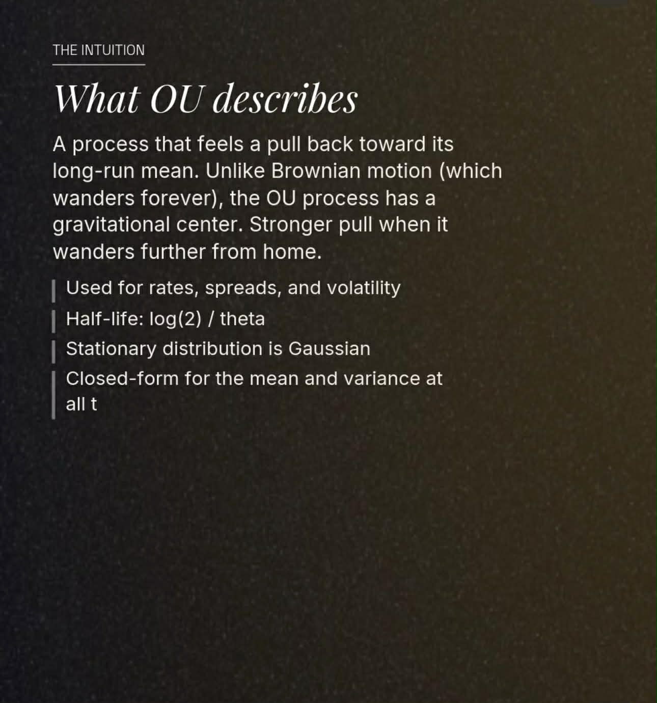
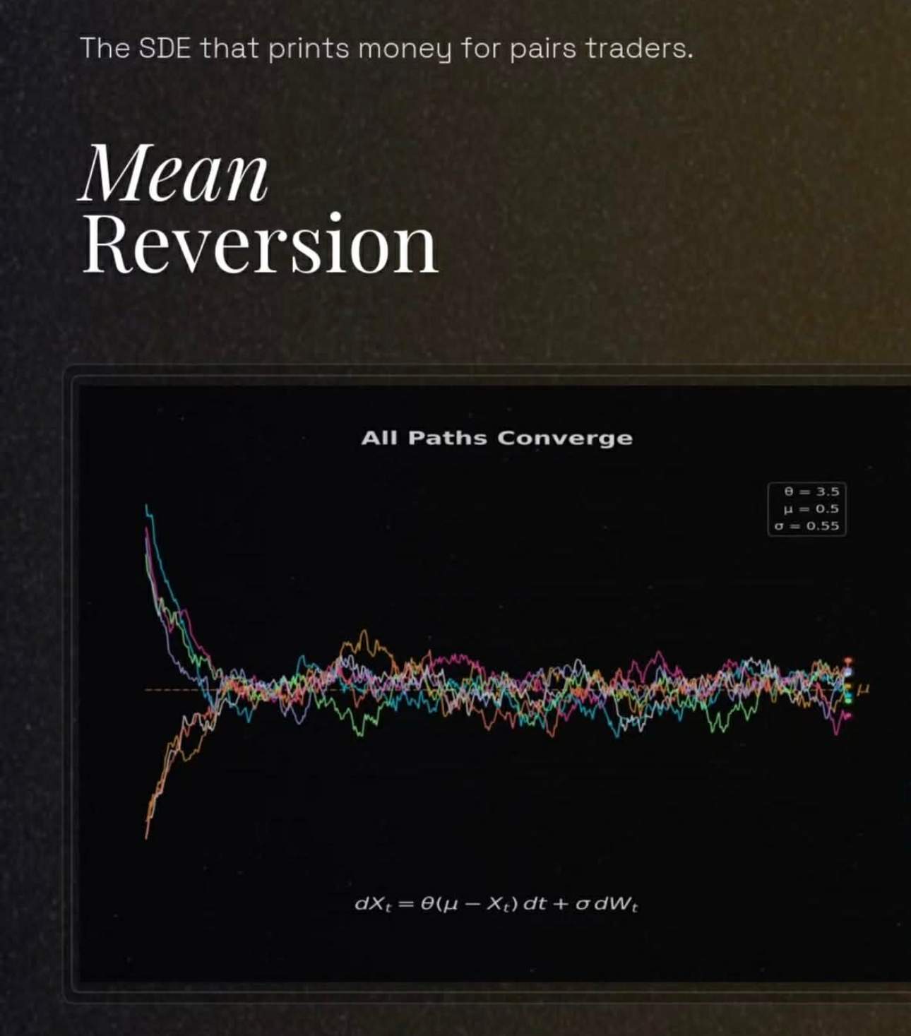
A process that feels a pull back toward its long-run mean. Brownian motion wanders; OU has a gravitational center. The farther the spread moves away from home, the stronger the pull becomes.
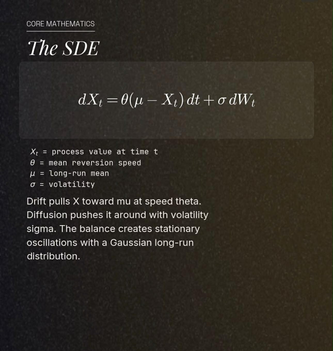
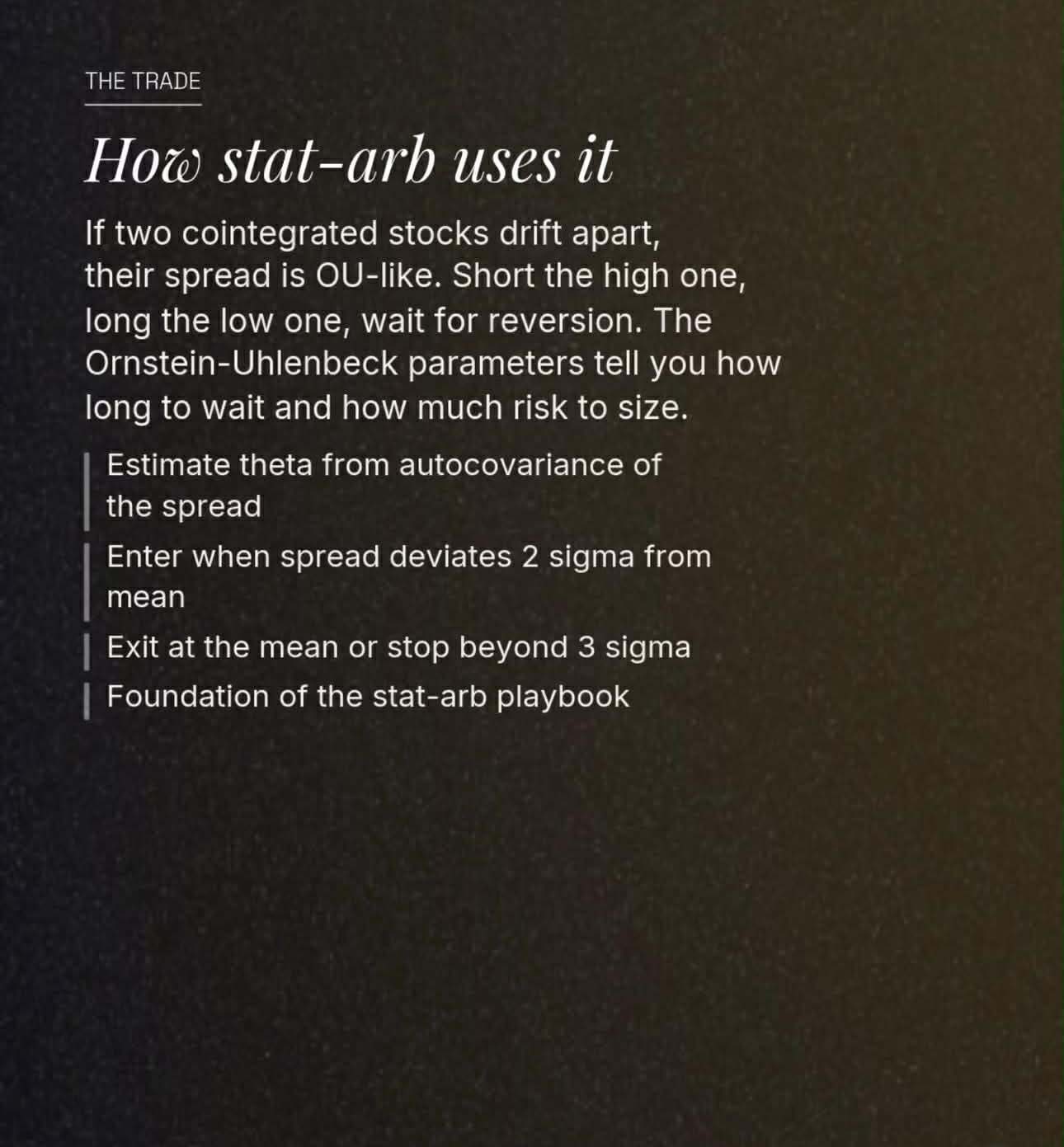
The Ornstein-Uhlenbeck process models a spread that gets pulled back toward a long-run mean. In stat-arb language: if two cointegrated assets drift apart, the spread can be traded as a spring, not as a random walk.
A process that feels a pull back toward its long-run mean. Brownian motion wanders; OU has a gravitational center. The farther the spread moves away from home, the stronger the pull becomes.
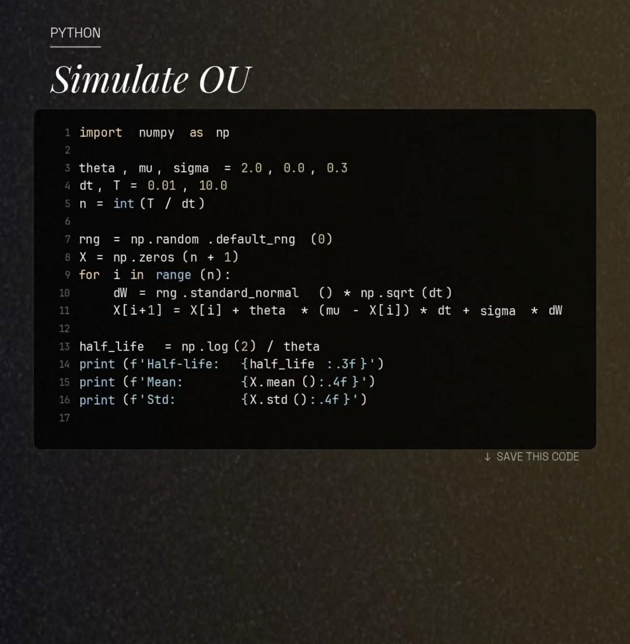
import numpy as np

theta, mu, sigma = 3.5, 0.5, 0.55
dt, T = 1 / 252, 1.0
n = int(T / dt)

rng = np.random.default_rng(0)
X = np.zeros(n + 1)
X[0] = 2.0

for i in range(n):
    dW = rng.standard_normal() * np.sqrt(dt)
    X[i + 1] = X[i] + theta * (mu - X[i]) * dt + sigma * dW

half_life = np.log(2) / theta
The live chart above is the same logic in browser form. The theta button increases mean-reversion speed, the stress button increases volatility and starting dispersion, and baseline keeps the classic stat-arb spread setup.